Cookbook
Cookbook.RmdIntroduction
This vignette contains sample code showing how to use the gsm extension gsm.simaerep using sample data from clindata.
In order to familiarize yourself with the gsm package,
please refer to the gsm
cookbook.
Load
suppressPackageStartupMessages(library(dplyr))
library(gsm.core)
library(gsm.mapping)
library(gsm.kri)
library(gsm.reporting)
library(gsm.simaerep)
#>
#> Attaching package: 'gsm.simaerep'
#> The following object is masked from 'package:gsm.kri':
#>
#>     MakeCharts
{gsm.simaerep} Functions
simaerep expects the cumulative count of numerator
events per denominator event per subject as input.
In this example we we are calculating the cumulative AE count per visit per patient per site.
dfInput <- Input_CumCount(
  dfSubjects = clindata::rawplus_dm,
  dfNumerator = clindata::rawplus_ae,
  dfDenominator = clindata::rawplus_visdt %>% dplyr::mutate(visit_dt = lubridate::ymd(visit_dt)),
  strSubjectCol = "subjid",
  strGroupCol = "invid",
  strGroupLevel = "Site",
  strNumeratorDateCol = "aest_dt",
  strDenominatorDateCol = "visit_dt"
)

dfInput %>%
  dplyr::filter(max(Numerator) > 1, .by = "SubjectID") %>%
  head(25) %>%
knitr::kable()| SubjectID | GroupID | GroupLevel | Numerator | Denominator |
|---|---|---|---|---|
| 0358 | 0X001 | Site | 0 | 1 |
| 0358 | 0X001 | Site | 0 | 2 |
| 0358 | 0X001 | Site | 0 | 3 |
| 0358 | 0X001 | Site | 0 | 4 |
| 0358 | 0X001 | Site | 0 | 5 |
| 0358 | 0X001 | Site | 1 | 6 |
| 0358 | 0X001 | Site | 1 | 7 |
| 0358 | 0X001 | Site | 1 | 8 |
| 0358 | 0X001 | Site | 1 | 9 |
| 0358 | 0X001 | Site | 1 | 10 |
| 0358 | 0X001 | Site | 2 | 11 |
| 0358 | 0X001 | Site | 2 | 12 |
| 0358 | 0X001 | Site | 2 | 13 |
| 0358 | 0X001 | Site | 2 | 14 |
| 0358 | 0X001 | Site | 5 | 15 |
| 0358 | 0X001 | Site | 5 | 16 |
| 0358 | 0X001 | Site | 6 | 17 |
| 0358 | 0X001 | Site | 6 | 18 |
| 0358 | 0X001 | Site | 7 | 19 |
| 0358 | 0X001 | Site | 7 | 20 |
| 0358 | 0X001 | Site | 7 | 21 |
| 0664 | 0X001 | Site | 0 | 1 |
| 0664 | 0X001 | Site | 0 | 2 |
| 0664 | 0X001 | Site | 0 | 3 |
| 0664 | 0X001 | Site | 0 | 4 |
Now we can analyze the data using Analyze_Simaerep() and
add flags with Flag_Simaerep() which adds a Score between
-1 and 1. Positive values indicate the over-reporting probability and
negative values indicate the under-reporting probability.
ExpectedNumerator is the number of expected AEs for a
site with the same patient configuration. ScoreMult is
Score with applied multiplicity correction.
dfAnalyzed <- Analyze_Simaerep(dfInput)
dfFlagged <- Flag_Simaerep(dfAnalyzed, vThreshold = c(-0.99, -0.95, 0.95, 0.99))
#> ℹ Sorted dfFlagged using custom Flag order: 2.Sorted dfFlagged using custom Flag order: -2.Sorted dfFlagged using custom Flag order: 1.Sorted dfFlagged using custom Flag order: -1.Sorted dfFlagged using custom Flag order: 0.


dfFlagged %>%
  arrange(Score) %>%
  head(25) %>%
knitr::kable()| GroupID | GroupLevel | Numerator | Denominator | Metric | Score | ScoreMult | ExpectedNumerator | Flag |
|---|---|---|---|---|---|---|---|---|
| 0X003 | Site | 4 | 276 | 0.0144928 | -1.000 | -1.0000000 | -41.979 | -2 |
| 0X043 | Site | 0 | 101 | 0.0000000 | -1.000 | -1.0000000 | -16.516 | -2 |
| 0X059 | Site | 14 | 312 | 0.0448718 | -1.000 | -1.0000000 | -38.485 | -2 |
| 0X080 | Site | 18 | 390 | 0.0461538 | -1.000 | -1.0000000 | -49.982 | -2 |
| 0X124 | Site | 35 | 596 | 0.0587248 | -1.000 | -1.0000000 | -67.513 | -2 |
| 0X126 | Site | 8 | 390 | 0.0205128 | -1.000 | -1.0000000 | -55.256 | -2 |
| 0X153 | Site | 25 | 597 | 0.0418760 | -1.000 | -1.0000000 | -74.767 | -2 |
| 0X161 | Site | 143 | 1442 | 0.0991678 | -1.000 | -1.0000000 | -98.937 | -2 |
| 0X163 | Site | 42 | 601 | 0.0698835 | -1.000 | -1.0000000 | -59.112 | -2 |
| 0X180 | Site | 12 | 261 | 0.0459770 | -0.999 | -0.9824000 | -32.029 | -2 |
| 0X026 | Site | 18 | 314 | 0.0573248 | -0.998 | -0.9729231 | -34.709 | -2 |
| 0X106 | Site | 1 | 107 | 0.0093458 | -0.998 | -0.9729231 | -17.200 | -2 |
| 0X157 | Site | 6 | 188 | 0.0319149 | -0.998 | -0.9729231 | -24.729 | -2 |
| 0X125 | Site | 11 | 230 | 0.0478261 | -0.996 | -0.9497143 | -29.653 | -2 |
| 0X016 | Site | 7 | 161 | 0.0434783 | -0.995 | -0.9450000 | -22.047 | -2 |
| 0X122 | Site | 23 | 352 | 0.0653409 | -0.995 | -0.9450000 | -36.143 | -2 |
| 0X160 | Site | 0 | 65 | 0.0000000 | -0.993 | -0.9275294 | -10.529 | -2 |
| 0X178 | Site | 12 | 221 | 0.0542986 | -0.992 | -0.9217778 | -23.114 | -2 |
| 0X129 | Site | 18 | 240 | 0.0750000 | -0.991 | -0.9208000 | -25.081 | -2 |
| 0X164 | Site | 0 | 80 | 0.0000000 | -0.991 | -0.9208000 | -13.117 | -2 |
| X187X | Site | 9 | 165 | 0.0545455 | -0.972 | -0.7680000 | -17.206 | -1 |
| 0X119 | Site | 4 | 107 | 0.0373832 | -0.971 | -0.7680000 | -13.469 | -1 |
| 0X088 | Site | 19 | 232 | 0.0818966 | -0.967 | -0.7536000 | -20.798 | -1 |
| 0X069 | Site | 4 | 96 | 0.0416667 | -0.966 | -0.7536000 | -12.778 | -1 |
| 0X100 | Site | 11 | 169 | 0.0650888 | -0.965 | -0.7536000 | -19.505 | -1 |
| GroupID | GroupLevel | Numerator | Denominator | Metric | Score | ScoreMult | ExpectedNumerator | Flag |
|---|---|---|---|---|---|---|---|---|
| 0X054 | Site | 33 | 47 | 0.7021277 | 0.996 | 0.8592 | 24.051 | 2 |
| 0X024 | Site | 74 | 140 | 0.5285714 | 0.999 | 0.9560 | 50.403 | 2 |
| 0X175 | Site | 129 | 366 | 0.3524590 | 0.999 | 0.9560 | 65.193 | 2 |
| 0X027 | Site | 93 | 210 | 0.4428571 | 1.000 | 1.0000 | 57.975 | 2 |
| 0X159 | Site | 397 | 695 | 0.5712230 | 1.000 | 1.0000 | 278.328 | 2 |
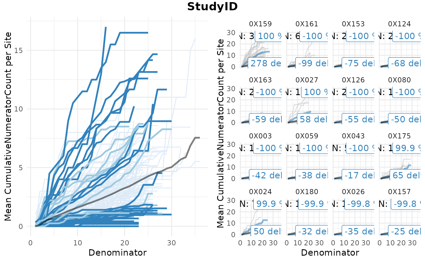
We can visualize the results as a ggplot or a htmlwidget
gsm.simaerep::Visualize_Simaerep(
  dfInput,
  dfFlagged
)
gsm.simaerep::Widget_Simaerep(
  dfInput,
  dfFlagged
)
gsm.kri::Widget_BarChart(
dfFlagged,
resultTooltipKeys = c(
"ExpectedNumerator",
"Score",
"Metric",
"Numerator",
"Denominator"
),
vOutcomeOptions = c(
"Score",
"Metric",
"Numerator",
"ExpectedNumerator"
)
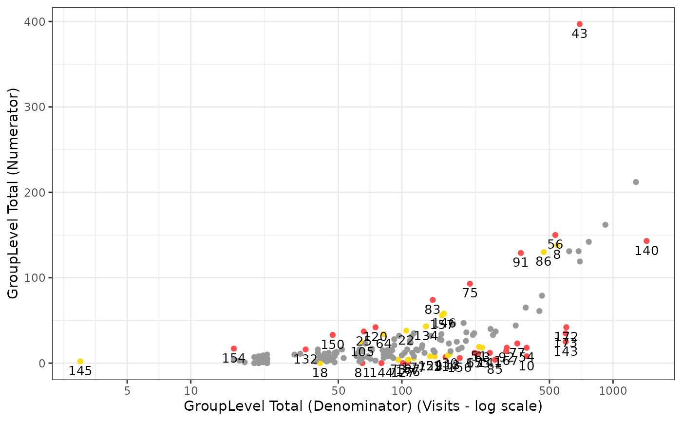
)These results are compatible with the gsm package for
visualization.
`simaerep scores represent are related to the metric ratio do not use a metric based threshold for flagging. Therefore we do not need to calculate boundaries to pass to the plotting function.
gsm.kri::Visualize_Scatter(
  dfFlagged,
  dfBounds = NULL,
  strGroupLabel = "GroupLevel",
  strUnit = "Visits"
)
Widget_ScatterPlot(
  dfFlagged,
  dfBounds = NULL,
  bDebug = FALSE,
  resultTooltipKeys = c(
    "ExpectedNumerator",
    "Score",
    "Metric",
    "Numerator",
    "Denominator"
  )
)
To compare we can also use the Score with applied multiplicity correction. For this we need to lower the threshold to be less sensitive to get a similar readout. Here we can see that overall the multiplicity correction dampens the score values and reduces the number of flagged sites. Simulation studies with {simaerep} have shown that multiplicity correction decreases detection rates. Nevertheless when monitoring a limited number of studies with many sites a sharper signal might be preferred.
dfFlagged_Mult <- Flag_Simaerep(
  dfAnalyzed %>%
    mutate(Score = ScoreMult),
  vThreshold = c(-0.95, -0.75, 0.75, 0.95)
)
#> ℹ Sorted dfFlagged using custom Flag order: 2.Sorted dfFlagged using custom Flag order: -2.Sorted dfFlagged using custom Flag order: 1.Sorted dfFlagged using custom Flag order: -1.Sorted dfFlagged using custom Flag order: 0.

Widget_BarChart(
  dfFlagged_Mult
)
Report Building
We can create a workflow to create the gsm KRI
report.
Mapping
lRaw <- list(
  Raw_SUBJ = clindata::rawplus_dm,
  Raw_AE = clindata::rawplus_ae,
  Raw_VISIT = clindata::rawplus_visdt,
  Raw_PD = clindata::ctms_protdev,
  Raw_ENROLL = clindata::rawplus_enroll,
  Raw_SITE = clindata::ctms_site,
  Raw_STUDY = clindata::ctms_study,
  Raw_SDRGCOMP = clindata::rawplus_sdrgcomp
)


mapping_wf <- gsm.core::MakeWorkflowList(
  strNames = NULL,
  strPath = system.file("workflow/1_mappings", package = "gsm.simaerep"),
  strPackage = NULL
)

lIngest <- gsm.mapping::Ingest(lRaw, gsm.mapping::CombineSpecs(mapping_wf))
#> Warning: Field `visit_dt`: 19 unparsable Date(s) set to NA

lMapped <- gsm.core::RunWorkflows(lWorkflows = mapping_wf, lData = lIngest)
Metrics
metrics_wf <- gsm.core::MakeWorkflowList(
  strNames = NULL,
  strPath = system.file("workflow/2_metrics", package = "gsm.simaerep"),
  strPackage = NULL
)

lAnalyzed <- gsm.core::RunWorkflows(lWorkflows = metrics_wf, lData = lMapped)
Report Generation - Workflow
reporting_wf <- gsm.core::MakeWorkflowList(
  strNames = NULL,
  strPath = system.file("workflow/3_reporting", package = "gsm.simaerep"),
  strPackage = NULL
)


lReport <- gsm.core::RunWorkflows(
  lWorkflows = reporting_wf,
  lData = c(
    lMapped,
    list(
      lAnalyzed = lAnalyzed,
      lWorkflows = metrics_wf
    )
  )
)

module_wf_gsm <- gsm.core::MakeWorkflowList(
  strNames = NULL,
  strPath = system.file("workflow/4_modules", package = "gsm.simaerep"),
  strPackage = NULL
)

# we cannot set a dynamic link to the report path in the yaml files
report_path <- system.file("report", "Report_KRI.Rmd", package = "gsm.simaerep")
n_steps <- length(module_wf_gsm$report_kri_site$steps)
module_wf_gsm$report_kri_site$steps[[n_steps]]$params$strInputPath <- report_path

lModule <- gsm.core::RunWorkflows(module_wf_gsm, lReport)
#> /opt/hostedtoolcache/pandoc/3.1.11/x64/pandoc +RTS -K512m -RTS /tmp/Rtmp03hd4O/Report_KRI.knit.md --to html4 --from markdown+autolink_bare_uris+tex_math_single_backslash --output /home/runner/work/gsm.simaerep/gsm.simaerep/vignettes/kri_report_AAAA0000000_Site_20260215.html --lua-filter /home/runner/work/_temp/Library/rmarkdown/rmarkdown/lua/pagebreak.lua --lua-filter /home/runner/work/_temp/Library/rmarkdown/rmarkdown/lua/latex-div.lua --embed-resources --standalone --variable bs3=TRUE --section-divs --table-of-contents --toc-depth 3 --variable toc_float=1 --variable toc_selectors=h1,h2,h3 --variable toc_smooth_scroll=1 --variable toc_print=1 --template /home/runner/work/_temp/Library/rmarkdown/rmd/h/default.html --no-highlight --variable highlightjs=1 --variable theme=bootstrap --css styles.css --include-in-header /tmp/Rtmp03hd4O/rmarkdown-str1c5d655a8780.html
Report Generation - Script
dfMetrics <- gsm.reporting::MakeMetric(lWorkflows = metrics_wf)

lAnalyzed <- gsm.core::RunWorkflows(lWorkflows = metrics_wf, lData = lMapped)


dfResults <- gsm.reporting::BindResults(
  lAnalysis = lAnalyzed,
  strName = "Analysis_Flagged",
  dSnapshotDate = Sys.Date(),
  strStudyID = "ABC-123"
)

dfInput <- gsm.reporting::BindResults(
  lAnalysis = lAnalyzed,
  strName = "Analysis_Input",
  dSnapshotDate = Sys.Date(),
  strStudyID = "ABC-123"
)

dfGroups <- dplyr::bind_rows(
  lMapped$Mapped_STUDY,
  lMapped$Mapped_SITE,
  lMapped$Country
)

dfBounds <- gsm.reporting::MakeBounds(
  dfResults = dfResults,
  dfMetrics = dfMetrics
)

lCharts_Rate <- gsm.simaerep::MakeCharts(
  dfResults = dfResults %>%
    filter(GroupLevel == "Site"),
  dfMetrics = dfMetrics %>%
    filter(GroupLevel == "Site", AnalysisType == c("rate", "binary")),
  dfGroups = dfGroups,
  dfBounds = dfBounds,
  bDebug = FALSE,
  strVisualizeFun = "gsm.kri::Visualize_Metric"
)

# we use a different tooltip for the simaerep charts
lCharts_Identity <- gsm.simaerep::MakeCharts(
  dfInput = dfInput %>%
    filter(GroupLevel == "Site"),
  dfResults = dfResults %>%
    filter(GroupLevel == "Site"),
  dfMetrics = dfMetrics %>%
    filter(GroupLevel == "Site", AnalysisType == "identity"),
  dfGroups = dfGroups,
  dfBounds = NULL,
  bDebug = FALSE,
  resultTooltipKeys = c(
    "ExpectedNumerator",
    "Score",
    "Metric",
    "Numerator",
    "Denominator"
  )
)

lCharts <- c(
  lCharts_Identity,
  lCharts_Rate
)

gsm.kri::Report_KRI(
  lCharts = lCharts,
  dfResults = dfResults,
  dfGroups = dfGroups,
  dfMetrics = dfMetrics,
  strOutputFile = "report_kri_site.html",
  strInputPath = system.file("report", "Report_KRI.Rmd", package = "gsm.simaerep")
)
#> /opt/hostedtoolcache/pandoc/3.1.11/x64/pandoc +RTS -K512m -RTS /tmp/Rtmp03hd4O/Report_KRI.knit.md --to html4 --from markdown+autolink_bare_uris+tex_math_single_backslash --output /home/runner/work/gsm.simaerep/gsm.simaerep/vignettes/report_kri_site.html --lua-filter /home/runner/work/_temp/Library/rmarkdown/rmarkdown/lua/pagebreak.lua --lua-filter /home/runner/work/_temp/Library/rmarkdown/rmarkdown/lua/latex-div.lua --embed-resources --standalone --variable bs3=TRUE --section-divs --table-of-contents --toc-depth 3 --variable toc_float=1 --variable toc_selectors=h1,h2,h3 --variable toc_smooth_scroll=1 --variable toc_print=1 --template /home/runner/work/_temp/Library/rmarkdown/rmd/h/default.html --no-highlight --variable highlightjs=1 --variable theme=bootstrap --css styles.css --include-in-header /tmp/Rtmp03hd4O/rmarkdown-str1c5d1a4cee39.html